Process Book
Tengis Kelley & Tyler Dinh · CSE 4507 Final Project
Overview and motivation
Janelia, working with Google Research, recently released the complete wiring diagram, or connectome, of a male fruit fly's central nervous system. It contains every neuron in the brain and nerve cord and the synapses between them. Google Research used AI to turn flat electron-microscope images into 3D reconstructions. That sped up the mapping enough that larger brains, and one day a human brain, now look possible to map.
A connectome records which neurons connect and how strongly. However, a connectome does not show what happens in the fly's nervous system when it smells vinegar or feels wind on its antennae. Fly Sense lets a user explore that question. A user picks one of the fly's five senses and a stimulus, such as an odor, a sound or a touch. The site switches on the matching sensory neurons and runs a simulation of the signal spreading through the network. A 3D view further helps to show and inspect the signal moving step by step until it reaches the output neurons that move the fly's body.
We had two motivations. The first was curiosity. People online had already wired the fly connectome into games like Doom and Flappy Bird, and we wanted to use the fly's own senses and body instead. The second was practical. In the proposal we hoped that knowing which stimuli drive which outputs could suggest better fly traps, for example by smell or by sweet versus bitter taste. We also hoped that comparing fly and human senses could point researchers at neuron groups worth studying. The Questions section explains the questions we set out to answer and how they changed.
The site covers smell, taste, hearing, sight and touch, with 19 stimuli taken from published studies. Each sense is a circuit of 2,200 to 5,100 neurons, which was parsed from the roughly 166,700 annotated neurons of the full dataset.
Related work
- The male CNS connectome. Our data comes from the Janelia male CNS v1.0 release. The Google Research announcement was a very popular thing to discuss upon its release.
- Fly connectome projects online. The awesome-fly list collects projects where a simulated fly brain plays Doom, Flappy Bird or Super Mario 64, drives a car or plays chess. These projects use the connectome as a controller for a game. For this project, we wanted the inputs and outputs to be the fly's own senses and body.
- Whole-brain simulation. Shiu et al. (2024, Nature) simulated the whole fly brain as spiking neurons on the connectome and predicted neurons involved in feeding. Their results convinced us that a simple model running on the wiring can give meaningful answers. Our model is a simpler rate model that runs in the browser (see Pruning and model decisions).
- Descending and motor neuron annotations. Cheong et al. (2024, eLife) define codes for the part of the nerve cord each descending neuron targets and the muscles each motor neuron drives. Our body-part labels come from these codes.
- Single-neuron behavior studies. Studies such as von Reyn et al. 2014 on the Giant Fiber and escape, and Bidaye et al. 2014 on the Moonwalker neuron and walking backward, give our tested behavior labels. Odor and sound studies give our stimuli. The Data and Pruning and model decisions sections cite each source where we use it.
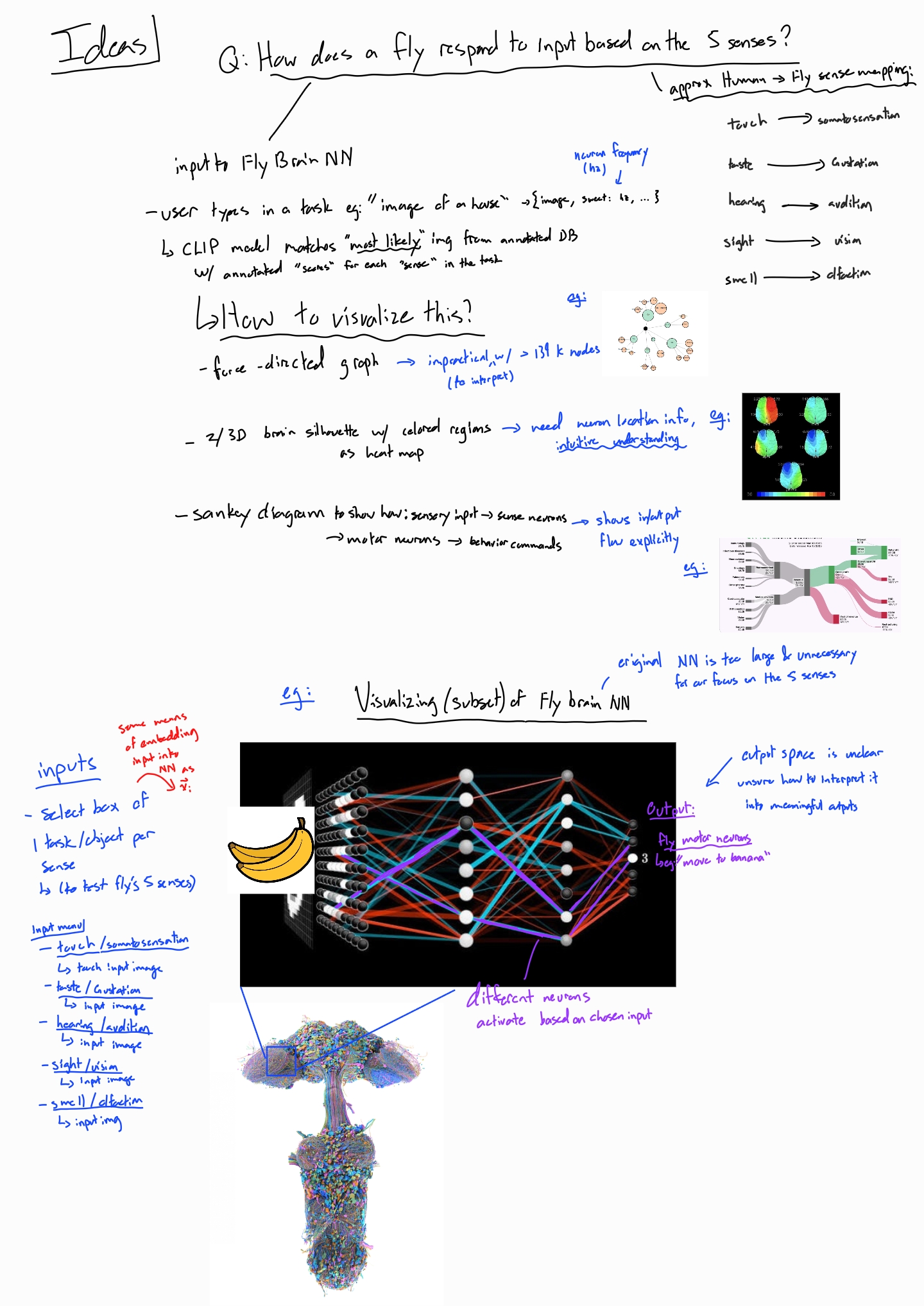
- Reference images in our sketches. The proposal sketches include images we collected online as inspiration. They show a layered neural-network diagram, Sankey and force-directed graph examples, and 3D renderings of the fly nervous system.
Questions
The proposal asked how a fruit fly's output neurons respond when one of its five senses receives a stimulus. We planned to read the answer as the fly's predicted state or feelings. We also planned two questions. What kind of trap would best lure a fly, if we vary its smell or its sweet or bitter taste? Could fly senses suggest neuron groups to study in humans?
Changed questions
- The predicted state or feelings of the fly eventually became more of a question about the fly's body parts. The connectome records no emotions, but it does record where each descending neuron sends its commands and which muscles each motor neuron moves. So the question we can answer is which body parts' circuits a stimulus drives, and how strongly.
- The trap question narrowed, because the dataset does not annotate taste receptors, so we cannot compare sweet and bitter. We define taste stimuli by body location instead.
New questions
- Do different stimuli (inputs) within one sense diverge and reach different outputs, or do they converge to similar outputs?
- Why are some senses much stronger than others? For example, smell outputs stay below about 0.13 activity, while taste reaches the maximum of 1.0.
- Where in the body does each circuit sit?
Data
Acquisition
We downloaded the full dataset, which are the three
files provided by the Janelia male CNS v1.0
release (minimum synapse confidence 0.5). The file scripts/download.py fetches them into
data/raw/, which is not committed to the GitHub repository because of its size.
| File | Size | Rows | What we use |
|---|---|---|---|
body-annotations | 14 MB | 211,577 bodies × 36 columns | superclass, class, subclass, type,
entryNerve, somaSide, somaLocation |
body-neurotransmitters | 43 MB | 1,835,518 bodies | consensus_nt (falling back to predicted_nt) |
connectome-weights | 1.05 GB | 151,856,684 connections | body_pre, body_post, weight (synapse count) |
Then, we keep the 166,700 elements that have a superclass annotation. That removes glia,
orphan fragments and unannotated pieces. Between these neurons, 6,242,118 connections have at least
5 synapses.
Annotations
In the proposal, we expected to search the literature to find which neurons belong to each sense. The provided annotations in the dataset made this much easier.
-
Every sense maps quite well onto the
classcolumn, so the sensory neurons for each sense are a single filter.Sense Filter Sensory neurons Smell class = olfactory2,639 (53 types, named by glomerulus, e.g. ORN_DA2)Taste class = gustatory1,428 (60 types; labellum, legs, wings, taste pegs, pharynx) Hearing class = mechanosensory,subclassauditory or wind_gravity589 (114 auditory + 475 wind/gravity, all in Johnston's organ) Sight class = visual6,091 photoreceptors (R1–R6, R7, R8 subtypes) Touch class = mechanosensory_tactile2,558 (56 types of bristle neurons) - The outputs are identifiable. There are 1,314 descending neurons (480 types) and 815 motor neurons (708 in the nerve cord, 107 in the brain). Descending neurons carry commands from the brain to the body, so they are the natural output layer. Some well-studied ones have known behaviors, such as the Giant Fiber for escape.
-
Neurons have 3D positions.
somaLocationgives x/y/z for 67% of bodies: nearly all central neurons (99% of central-brain neurons, 100% of descending neurons), but none of the sensory neurons, whose cell bodies sit outside the CNS. In the proposal we had listed the brain heat map (Design Option 2) as blocked by missing positions, but this ends up unblocking it. - Olfactory types map to known odors. Because they are named by glomerulus, published odor–glomerulus findings apply directly. For example, geosmin activates only DA2 (Stensmyr et al. 2012).
Limitations
-
Taste cannot be split into sweet and bitter. Receptor identity is not annotated:
receptorTypehas only three putative labels (ppk23, ppk25, IR52b) on about 750 neurons, and none of them are sugar or bitter receptors. Taste stimuli are therefore defined by body location. - Sight is very large. 6,091 photoreceptors feed an optic lobe of about 89,000 local neurons, so the sight circuit needs a deeper and more selective pruning than the other senses (see Pruning and model decisions).
- Sensory neurons have no position. We place each one at the synapse-weighted mean position of the neurons it connects to.
Stimuli
In the proposal, a CLIP model would turn a typed prompt into an input vector. For this milestone we use hand-picked presets instead: each one switches on a specific group of sensory neurons, chosen from the published literature. We checked every citation against the original papers and dropped the ones that did not hold up. For example, our first vinegar preset also included the DM4 and DP1m glomeruli. Neither is supported for vinegar, so the preset now uses only DM1 and VA2, as Semmelhack & Wang (2009) show.
| Sense | Stimulus | Sensory neurons switched on | Basis |
|---|---|---|---|
| Smell | Apple cider vinegar | ORN_DM1, ORN_VA2 (156) | Semmelhack & Wang 2009 |
| Geosmin (mold) | ORN_DA2 (46) | Stensmyr et al. 2012 | |
| CO₂ (fly stress odor) | ORN_V (54) | Suh et al. 2004 | |
| cVA (male pheromone) | ORN_DA1 (184) | Kurtovic et al. 2007 | |
| Taste | Mouth (labellum) touches food | labellar bristle (147) | Engert et al. 2022 (anatomy) |
| Legs step onto food | leg bristle (608) | dataset subclass | |
| Swallowing (pharynx) | pharyngeal sensillum (48) | dataset subclass | |
| Taste pegs | taste peg (58) | dataset subclass | |
| Hearing | Courtship song (low frequency) | JO-B (87) | Kamikouchi et al. 2009; Matsuo et al. 2014 |
| High-frequency vibration | JO-A (50) | Kamikouchi et al. 2009; Matsuo et al. 2014 | |
| Wind gust / gravity | JO-C/E (475) | Yorozu et al. 2009 | |
| Sight | Bright flash / looming shadow | R1–R6 (256) | motion and luminance photoreceptors |
| UV light | R7 (377) | R7 express UV opsins Rh3/Rh4 | |
| Blue light | R8p (87) | R8p express blue opsin Rh5 | |
| Green light | R8y (107) | R8y express green opsin Rh6 | |
| Touch | Front leg touched | bristles entering by the prothoracic leg nerve (120) | dataset entryNerve |
| Hind leg touched | bristles entering by the metathoracic leg nerve (432) | dataset entryNerve | |
| Back (notum) touched | notum bristles (200) | dataset subclass | |
| Whole body brushed | all tactile bristles in the circuit (1,238) | dataset class |
Counts are the neurons a stimulus switches on in the built circuit. Large sensory groups are sampled (see Pruning and model decisions). Some counts are larger than a circuit's input layer: sensory neurons also synapse onto each other, so the pruning adds some of them at deeper layers, and a stimulus switches those on too. "Whole body brushed" turns on 1,238 tactile neurons; 623 are in the input layer and the rest sit in layers 1–6.
Data structures
The file scripts/build_subgraphs.py turns the raw files into one JSON file per sense in
data/processed/, plus meta.json, which lists the senses, the pruning
parameters, the simulation constants and the behavior labels. The website reads only these files.
All five senses are built:
| File | Neurons | Connections | Layers | Inputs | Outputs | Size |
|---|---|---|---|---|---|---|
smell.json | 2,541 | 20,915 | 7 | 628 | 164 | 1.5 MB |
taste.json | 2,530 | 24,755 | 7 | 604 | 263 | 1.7 MB |
hearing.json | 2,203 | 20,224 | 7 | 589 | 237 | 1.4 MB |
sight.json | 5,124 | 26,005 | 11 | 601 | 126 | 2.3 MB |
touch.json | 2,611 | 18,873 | 7 | 623 | 260 | 1.5 MB |
Each sense file has the same structure:
{
  "sense": "smell", "label": "Smell (olfaction)",
  "sim":   { "steps": 9, "decay": 0.5, "gain": 4.0 },
  "nodes": [{ "id", "type", "superclass", "class", "side", "nt",
              "sign",       // +1 excitatory, -1 inhibitory, 0 modulatory
              "layer",      // hops from the sensory input (0 = input)
              "role",       // input | hidden | output
              "pos",        // normalized soma x/y/z
              "behaviour",       // output label (see Output labels)
              "behaviour_basis", // "literature" | "target"
              "region" }],       // body part, e.g. "front_leg"
  "edges": [{ "s", "t", "w",   // w = synapse count
              "wn",            // w / all synapses onto t
              "sign" }],
  "stimuli":   [{ "id", "label", "valence", "source", "neurons": [ids] }],
  "reference": { "<stimulus id>": { "top_outputs": [...] } }
}
reference stores the Python simulation's result for every stimulus. The website's
JavaScript simulation is checked against it (all 19 stimuli match).
Pruning and model decisions
Our proposal noted that the whole CNS dataset would be too large to show or simulate in a browser, so we would fix this by cutting out
one circuit per sense. This section covers how we implemented the pruning and how a stimulus can travel through the
circuit. All settings are in the file scripts/config.py.
The circuit
- Inputs (layer 0). The sensory neurons of the sense, at most 600. Larger groups are sampled in proportion to each cell type, and the neurons used by a stimulus preset get priority, so small presets keep all their neurons.
- Grow outward one layer at a time, up to 6 layers (10 for sight). A downstream neuron is kept if at least 3% of all the synapses it receives come from neurons already in the circuit, and each layer keeps the 450 highest-scoring ones. Connections with fewer than 5 synapses are ignored.
- Reserve room for the outputs. Descending and motor neurons collect input from many places, so a sense rarely provides 3% of it. They get a separate budget (80 per layer) and a lower threshold (1%).
- One budget per stimulus. Each stimulus is grown separately with its share of the budget, and the results are merged. In our first version all stimuli shared one budget. The strongest stimulus then took every slot: geosmin and CO₂ were left with no path to any output.
- Thin the connections. Each neuron keeps its 12 strongest incoming connections, so the browser draws about 19,000–26,000 lines per sense instead of every connection.
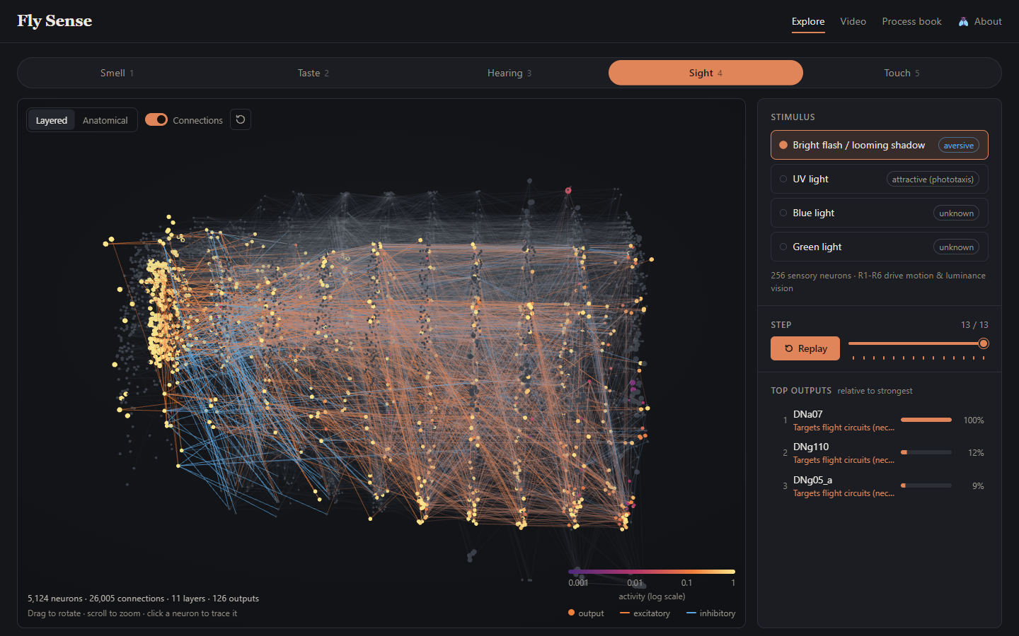
Sight needed extra work. The optic lobe is so dense that, with 6 layers, the circuit never left it and reached zero outputs. With 10 layers it reached one. Visual projection neurons carry signals out of the optic lobe, so we gave them the same reserved budget as the outputs. The sight circuit now reaches 126 outputs over 11 layers.
Connections
| Neurotransmitter | Sign | Reason |
|---|---|---|
| Acetylcholine | +1 | The main excitatory transmitter in flies |
| GABA, glutamate | −1 | Inhibitory (glutamate acts mainly through inhibitory GluCl channels in flies) |
| Histamine | +1 | Used by photoreceptors. Strictly it is inhibitory, but treating it as −1 would stop all visual signals at the first synapse in our model. |
| Dopamine, serotonin, octopamine | 0 | Modulators. They change how circuits respond rather than passing a signal, which our model cannot represent. |
Sensory neurons always pass their signal on (+1). Each connection's strength is its synapse count divided by all synapses the receiving neuron gets anywhere in the CNS, including weak connections and unannotated fragments. A value of 0.2 in simpler terms is then "this input supplies 20% of all the synapses the receiving neuron gets".
Model
We use a simple rate model. It was inspired by the whole-brain model of Shiu et al. (2024, Nature), which simulated spiking neurons over the fly connectome to predict feeding behavior; ours tracks only an average activity per neuron. Every neuron has an activity between 0 and 1:
start:      r = 1 for stimulated neurons, 0 for all others
each step:  input_j = Σ over connections i→j of  sign_i × strength_ij × r_i
            r_j     = clamp(0.5 × r_j + 4 × input_j, 0, 1)
            stimulated neurons stay at 1
The simulation runs for at least 8 steps, and for 2 more steps than the circuit has layers, so the
signal can reach the last layer (9 steps for most senses, 13 for sight). Every step is kept so the
website can animate the signal moving through the network. The same model runs in Python
(simulate() in scripts/build_subgraphs.py) and in the browser
(js/simulate.js), and the two agree to within 0.0001 on all 19 stimuli.
Gain
The gain (4) sets how strongly activity is passed on. We tried several values on an earlier version of the circuits (10 steps each), and no single value suited every sense:
| Gain | Smell, vinegar: strongest output | Taste, labellum: outputs above 0.1 |
|---|---|---|
| 3 | 0.05 | 23 |
| 5 | 0.25 | 166 |
| 8 | 0.49 | 248 |
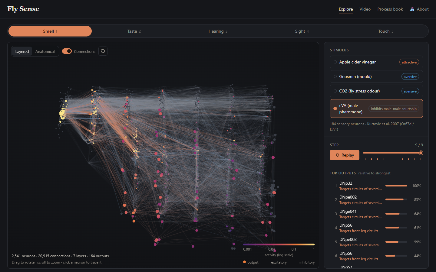
At gain 8, smell finally produces clear outputs, but taste is saturated, with hundreds of outputs lit up. We chose a moderate gain, and the website shows each output's activity relative to the strongest output of the current run instead of on a fixed 0–1 scale. With the current circuits, smell's strongest outputs reach only 0.003–0.13, while taste and wind reach 1.0.
Predictions
The strongest output for each stimulus, from reference in the data files:
| Sense | Stimulus → strongest outputs (activity) |
|---|---|
| Smell | vinegar → DNb05 (0.048), DNc01 (0.047) · geosmin → DNp29 (0.003) · CO₂ → DNp29 (0.053) · cVA → DNp32 (0.128) |
| Taste | labellum → DNg67 (1.0) · legs → DNg103 (0.83) · pharynx → MN10, a mouthpart motor neuron (0.96) · taste pegs → DNge098 (0.68) |
| Hearing | song → DNge111 (0.38) · vibration → DNg09_a (0.85) · wind → DNge091, DNge111 (1.0) |
| Sight | flash → DNa07 (0.029) · UV, blue, green → DNpe011 (0.028–0.039) |
| Touch | front leg → leg motor neurons (Tr flexor 0.13) · hind leg → sternal rotator motor neuron (0.09) · back → DNg20 (0.28) · whole body → DNge122 (0.46) |
Different stimuli within a sense mostly drive different outputs, which is the core idea of the project. However, sight is the exception, with UV, blue and green all peaking at the same neuron, DNpe011.
Output labels
Outputs get one of two kinds of label, and our data files record which kind in
behaviour_basis.
1. Tested behaviors ("literature"). We gave these only to output neurons
whose behavior has been shown experimentally, and checked each source:
| Cell type | Behavior | Source |
|---|---|---|
| DNp01 (Giant Fiber) | Escape takeoff | von Reyn et al. 2014 |
| MDN (Moonwalker) | Walk backward | Bidaye et al. 2014 |
| DNg100 (BDN2) | Walk forward | Pugliese et al. 2025 |
| DNp09 (P9) | Walk forward / approach | Bidaye et al. 2020 (as "P9"; that P9 is DNp09 is likely but not confirmed) |
| DNa01, DNa02 | Turn / steer | Rayshubskiy et al. 2025 (DNa02 well supported; DNa01's role is less certain) |
| DNg62, DNge078 (aDN1, aDN2) | Groom antennae | Hampel et al. 2015 |
| MN9 | Extend proboscis (feed) | Gordon & Scott 2009; Shiu et al. 2024 |
We observe that the Giant Fiber and the grooming neurons show up in hearing, MN9 and the grooming neurons in taste, MN9 in smell, and the grooming neurons in touch. However, none rank in the top 10 outputs for any stimulus, and sight contains none of them. With only these labels, the outputs panel showed bare cell type names.
2. Body-part targets ("target"). Every other output is labeled with a body part using the dataset's annotations. This doesn't describe a tested behavior, so the labels say "Targets…" or "Moves…" rather than naming an action.
| Output | Annotation used | Example labels |
|---|---|---|
| Descending neurons | subclass: the region of the nerve cord the neuron targets |
"Targets front-leg circuits", "Targets flight circuits (neck, wing, haltere)", "Targets wing + leg coordination (takeoff, landing)", "Targets several motor systems" |
| Nerve-cord motor neurons | subclass: the muscle group |
"Moves the front leg", "Moves the wing", "Moves the abdomen" |
| Brain motor neurons | exitNerve: the nerve the axon leaves through |
"Moves the mouthparts (pharyngeal nerve)", "Moves the antenna" |
The descending and motor neuron codes are defined by Cheong et al. (2024, eLife), who also
describe the upper tectulum as a single flight motor system and the lower tectulum as a hub for
behaviors that need wings and legs together, such as takeoff. We found no paper defining the codes for
brain motor neurons, so for those we used the exit nerve: the pharyngeal and labial nerves supply the
mouthparts, the antennal nerve the antenna, and the cervical nerve the neck. That mapping is our
inference from nerve anatomy. Each label also has a region key (for example
front_leg, flight, mouthparts), so the website can light up the
matching part of a fly body.
With both kinds, 1,038 of the 1,050 outputs across the five circuits have a label, and so do 172 of the 174 top-10 outputs that receive any activity. The labels also give a sanity check on the model. Touching the front leg most strongly drives motor neurons that move the front leg. Touching the hind leg drives hind-leg motor neurons. Swallowing drives a mouthpart motor neuron, and wind and a bright flash both drive descending neurons that target flight circuits.
The weakness is that the most common label for descending neurons, "Targets several motor systems", doesn't offer too much information. Linking these outputs to specific behaviors would be the main open problem for the next milestone.
Exploratory data analysis
First, we looked at the dataset tables to learn what the annotations could give us. Then, we built the circuits and looked at them in early versions of the explorer.
| What we looked at | What we found | What it changed |
|---|---|---|
Neuron counts by class and subclass |
Each sense maps to one annotation filter (see the table in Data) | We did not need a literature search to find sensory neurons, so the time went into choosing stimuli. |
Coverage of somaLocation |
67% of neurons have a 3D position. Nearly all central neurons have one, but no sensory neurons do. | The anatomical heat map from proposal Option 2 became possible. We place sensory neurons at their partners' mean position. |
receptorType values for taste neurons |
No sugar or bitter receptor labels | Taste stimuli use body location, and we dropped the sweet versus bitter trap question. |
| Output neurons with a known behavior | Only 9 cell types, and none in any top 10 | We added body-part labels, and the outputs list styles them apart from tested behaviors. |
| First sight circuit (6 layers) in the layered view | The signal never left the optic lobe and reached zero outputs | Sight now has 11 layers and a reserved budget for visual projection neurons. |
| Gain | No single gain suits every sense. Smell stays faint while taste saturates. | Activity colors use a log scale, and output bars are relative to the strongest output. |
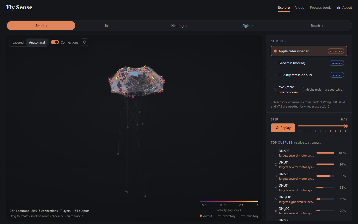
| Anatomical layout of each circuit | 85% of the touch circuit is in the nerve cord, and nearly all of the smell circuit is in the brain | We kept the anatomical layout as a full view next to the layered one. |
Design evolution
Proposal sketches
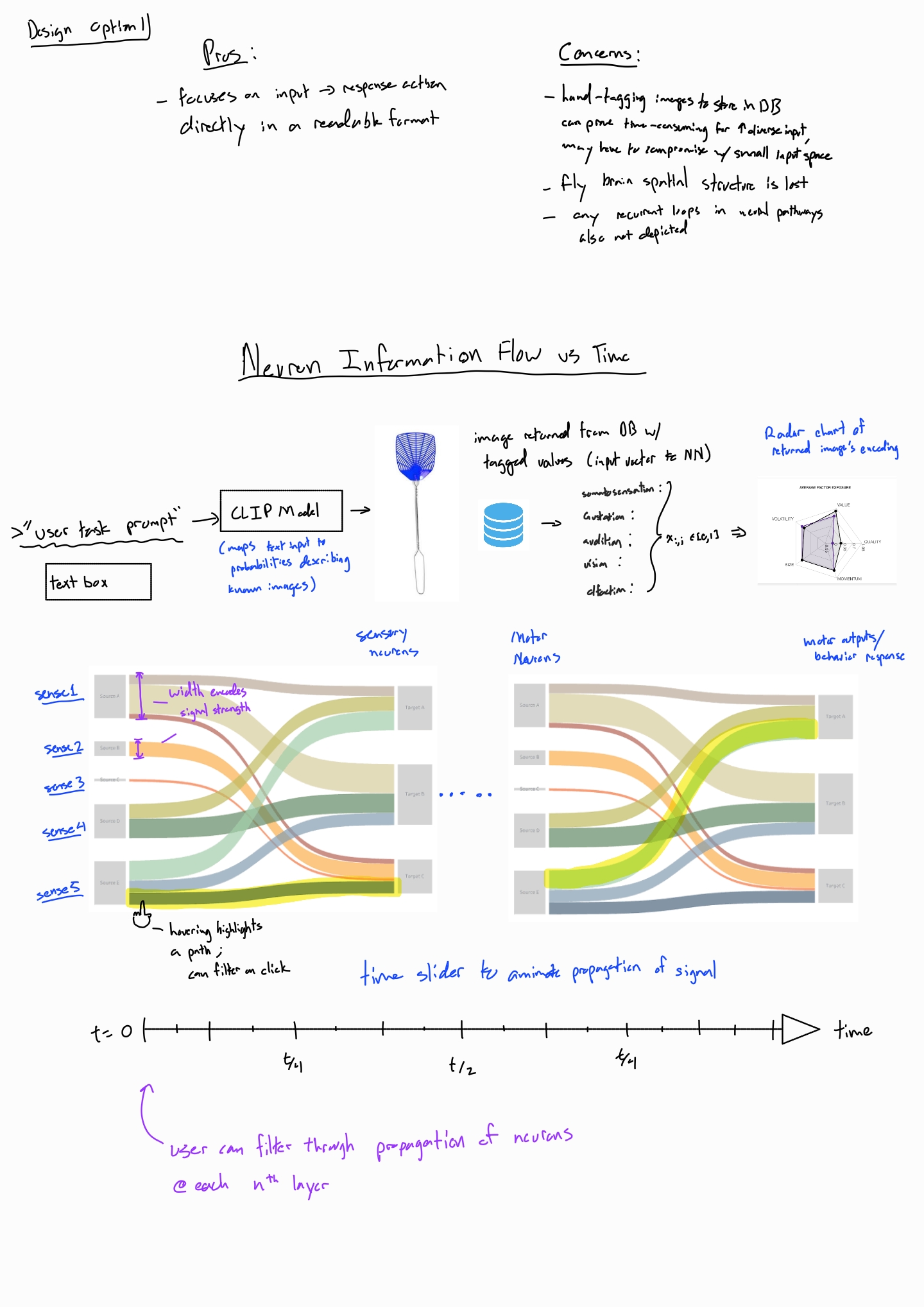
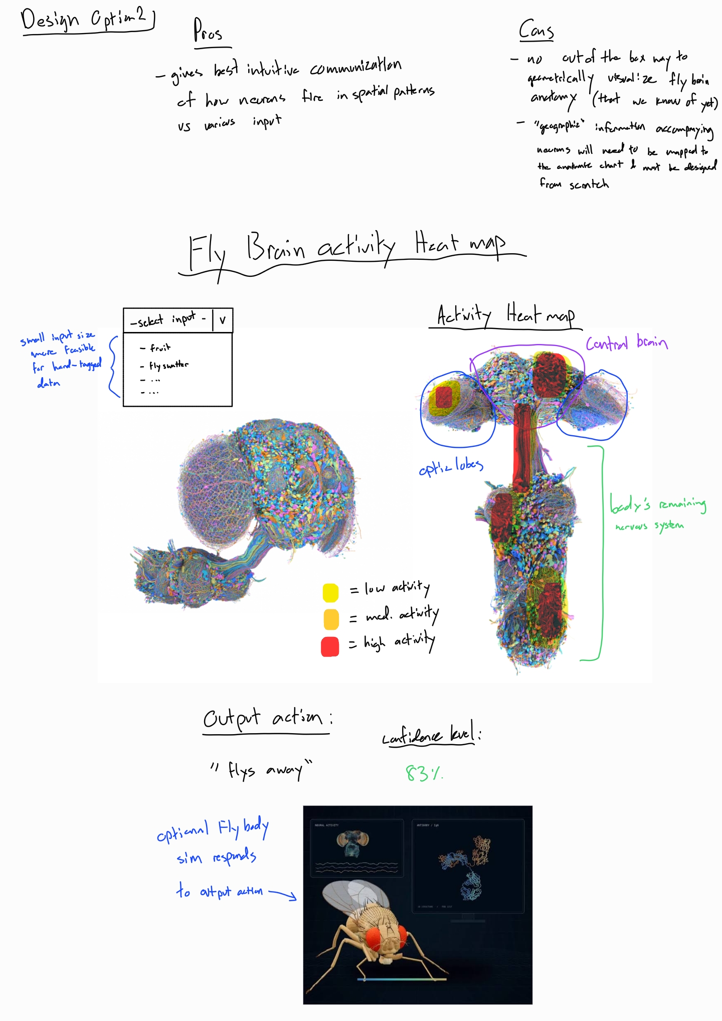
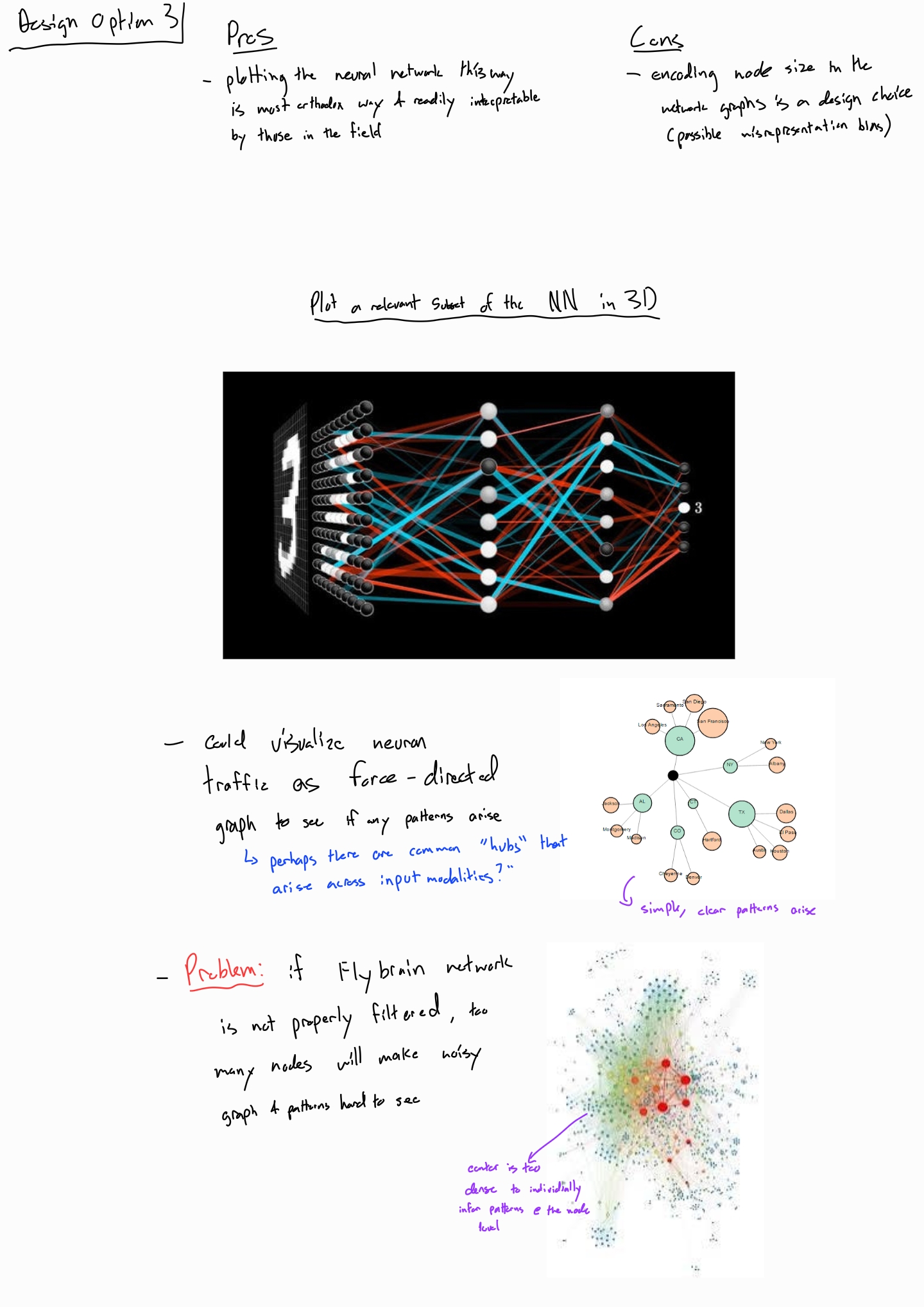
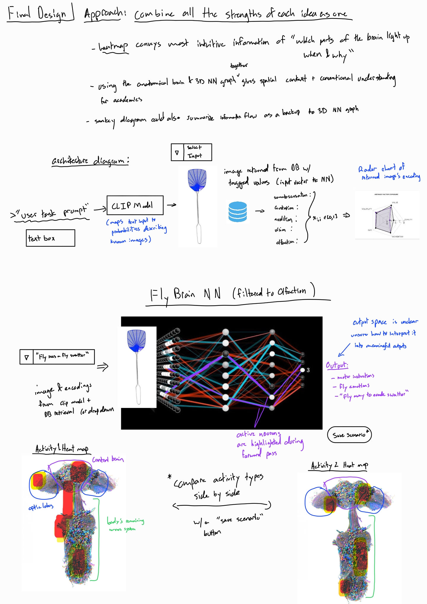
The proposal explored three directions and then combined them. Click a sketch to open it at full size.
Proposal vs current
| Proposal | Now | Why |
|---|---|---|
| Typed prompt matched by CLIP to a tagged image | A list of 19 preset stimuli, grouped by sense | Each preset switches on specific sensory neurons and cites a published source. A per-sense CLIP score would not be able to determine which neurons to switch on, and tagging images by hand is infeasible. |
| Radar chart of the input vector | Dropped. A short description sits under the stimulus list. | Each stimulus belongs to one sense, so there is no multi-sense vector to show. |
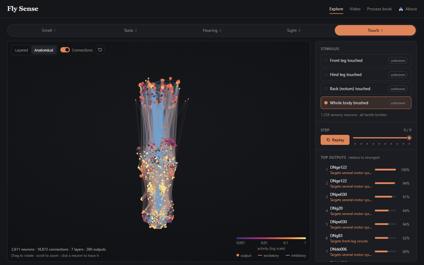
| 3D layered network (Option 3) | Kept as the Layered layout | The x axis counts hops from the input, so position shows how far a signal has traveled. |
| Anatomical heat map (Option 2) | Kept in 3D as the Anatomical layout | Soma positions made it possible. Both layouts use the same neurons and colors, and switching animates each neuron to its new position, so you can follow it. |
| Sankey diagram (Option 1) | Not built | The 3D views and the step slider already show the flow over time. |
| Readable action or feeling with a confidence | A ranked list of output neurons with labels | The data supports body-part targets, not emotions or confidence. See Questions. |
| "Save Scenario" comparison | Not built | The URL records the sense, stimulus and layout, so two runs can be opened in separate tabs. A built-in side-by-side view is future work. |
| Hover tooltips and drag to rotate | Built | Tooltips show cell type, label, role, layer, neurotransmitter and activity. |
Design decisions
- Activity uses a log-scale sequential color ramp. It runs from dark purple through magenta and orange to pale yellow, like the magma color map. Activity spans three orders of magnitude, from 0.001 to 1, so a linear scale would leave smell almost black. Lightness rises steadily with activity, so the order reads correctly even in grayscale. Silent neurons are neutral gray, outside the ramp.
- Hue shows connection sign. Excitatory connections are orange and inhibitory ones are blue. Sign is a category, so it gets hue instead of lightness. Orange and blue stay distinct to address concerns posed by color blindness.
- Silent connections are nearly invisible. They draw at 2.5% opacity, because twenty thousand lines at full strength would be unreadable. The faint lines keep the circuit's shape as context. Active connections take their sign color, with opacity scaled by activity times connection strength.
- Size shows role only. The proposal worried that node size can imply importance, so size encodes one category and never activity. Outputs are larger than other neurons, which makes the end of each pathway easier for the user to find.
- Output strength is bar length on a shared baseline. Each bar is relative to the run's strongest output, with the percentage printed beside it. Cleveland and McGill found that position and length on a common scale are the most accurately judged encodings. The relative scale keeps faint senses readable.
- We follow the principle of providing the overview first, and providing details on demand. So, the layout tries to follow Shneiderman's mantra. Sense tabs and the stimulus list give the overview, and the 3D view and outputs list show the result. Clicking a neuron dims everything unrelated and opens its details.
Implementation
The site is static HTML, CSS and JavaScript modules, with no build step. The Python pipeline writes one
JSON file per sense. The browser loads that file, runs the simulation in js/simulate.js and
draws the result with three.js in js/network3d.js.
Interface
- Sense tabs. Keys 1 to 5 also switch senses. The old circuit fades out and the new one grows in layer by layer.
- Stimulus list. Each stimulus shows its valence, and the selected one shows how many sensory neurons it switches on. Choosing a stimulus runs the simulation and plays it.
- Playback. Play and pause (Space) advance one step per second, and the slider or arrow keys (Left, Right) help to move forward or backward to any step. The colors flow in the network between steps, to indicate more of a continuous motion to the user.
- 3D network. Drag to rotate, right-drag to pan and scroll to zoom. A switch changes between the Layered and Anatomical layouts (L), a toggle hides connections (C), and a button resets the camera (R). The legend shows the activity scale and the connection colors.
- Hover. Hovering a neuron shows its cell type, label, role, layer, neurotransmitter and activity.
- Top outputs. The list shows the 10 most active output neurons and ranks them continuously with a smooth reorder at every step. Hovering a row draws a ring around the same neuron in the 3D view, and clicking it selects the neuron and moves the camera to it.
- Neuron details. Selecting a neuron dims the rest of the circuit and replaces the outputs list with its details. These are an activity sparkline over the run and the neuron's four strongest inputs and targets. Clicking an input or target selects it, so you can trace a signal backward or forward.
- About. The About panel (A) explains the page and lists every control.
Evaluation
- Stimuli within a sense mostly reach different outputs. In smell, vinegar, CO2 and cVA each peak at a different descending neuron, and so do song, vibration and wind in hearing. This helps to provide some evidence towards an answer to our question, predicting that within-sense stimuli have different outputs.
- The wiring reaches the expected body parts. Touching the front leg drives motor neurons that move the front leg, and touching the hind leg drives hind-leg motor neurons. Swallowing drives a mouthpart motor neuron. Wind and a bright flash drive descending neurons that target flight circuits. We did not build any of this into the model, so it is a useful sanity check.
- Senses differ a lot in strength. Taste and wind reach the maximum activity of 1.0, while smell and sight stay below 0.13. The cVA pheromone is the strongest smell, at 2.7 times the activity of vinegar.
- Circuits sit in different places. In the anatomical layout, nearly all of the smell circuit is in the brain, while 85% of the touch circuit is in the nerve cord.
Future improvements
- A simulated physical fly body figure that lights up the targeted body parts, or moves it around in a simulated environment.
- A side-by-side comparison of two stimuli.
- A stronger geosmin circuit / network. Currently, only one output neuron receives any activity.
- Better labels for the descending neurons that target "several motor systems".
Generative AI use
From the course policy:
"…Generative AI may be used for the final project. When generative AI is permitted and contributes meaningfully to your work, disclose that use as directed. Regardless of whether AI assistance is permitted, you remain responsible for understanding, testing, evaluating, and being able to explain the work you submit.
Required WashU academic integrity statement
In all academic work, the ideas and contributions of others (including generative artificial intelligence) must be appropriately acknowledged and work that is presented as original must be, in fact, original…"
We used AI coding agents (Claude) during this project to spend less time on tedious coding, writing, and debugging and much more on designing the visualization and the user experience. We both have experience with agentic coding, so we worked with the agents extensively to design and plan features. We also tried a multi-agentic message board approach for the first time, which can be seen in a GitHub issue in our repository (issue #1) where our two agents posted their progress and questions for each other.
We reviewed, tested, and finalized all work, and we can explain it. As a sanity check, the browser simulation matches the Python simulation on all 19 stimuli.
Data / Processing (Tengis's agent)
-
Data pipeline. The agent helped write the pipeline in
scripts/that builds the per-sense circuits. -
Citation check. The agent checked every literature source behind the stimulus presets
and behavior labels in
scripts/config.pywith web searches. We dropped or corrected the sources that did not hold up, and the agent posted every change to the message board before it went into the process book. -
Output labels. The agent added coarse body-part labels for descending and motor
neurons (
behaviour_basis: "target"), using the dataset's annotation codes as Cheong et al. (2024) define them. For brain motor neurons, the mapping from exit nerve to body part is the agent's inference from nerve anatomy, andscripts/config.pymarks it as such. -
Process book. The agent drafted the Data and Pruning and model decisions sections from
the generated data files and measured runs. It also captured the screenshots in
img/processbook/from the explorer with a headless browser.
Frontend (Tyler's agent)
-
Website. The agent helped build the explorer in
index.html,css/andjs/, including the three.js network view, playback, the outputs list and the neuron details. -
Simulation port. The agent ported the forward pass to
js/simulate.jsand checked it against the Python reference for all 19 stimuli. - Output labels in the interface. The agent shortened the body-part labels in the outputs list and styled them apart from tested behaviors.
- Process book. The agent drafted the Overview, Related work, Questions, Exploratory data analysis, Design evolution, Implementation and Evaluation sections from the proposal and the project files.