Turn The Light On: Light Pollution Associated with Health Risks and Outcomes
MJ Hong (hong.m.j@wustl.edu, 520521)
Gabi Wurgraft (g.t.wurgaft@wustl.edu, 499038)
Mia Hines (hines.mia@wustl.edu, 526493)
Overview and Motivation.
We are curious about how the modern world is shaping the health of its people. While many technological and societal advancements result in longer, more fulfilling lives than before, they can cause some adverse effects. Originally, we were considering the effects of noise pollution, light pollution, or green spaces on the health of individuals. The growth of big cities has caused a large increase in artificial light to shine at all hours of the day and night. There has also been an increase in noise pollution due to population density and technological advancements. In an attempt to curb the negative effects of different kinds of pollution, green spaces are recommended to improve individuals’ health. Ultimately, we decided to focus on light pollution and its effects on both physical and mental health. We chose light pollution because the topic had cleaner and more robust datasets than those of green spaces and sound pollution.
Personal backgrounds are attached to the research topic. Some of us have come from a more rural area and moved to St Louis. The bright lights shining all the time are a big adjustment from the darker rural areas, where nighttime is clearly distinguished from daytime. It was a big adjustment, and through that experience, we wondered if all this artificial light could negatively affect a resident’s health. We decided to frame it on a national scale, instead of just St. Louis, to see how different levels of light pollution can affect sleep and mental health.
Related Work.
We were inspired by the paper Missing the Dark: Health Effects of Light Pollution [1], that talks about the connection between artificial light and sleep disorders.
We were also inspired by the paper Insights into the Effect of Light Pollution on Mental Health: Focus on Affective Disorders–A Narrative Review [2], which draws a conenction between mental health and artificial light.
- Chepesiuk R. Missing the dark: health effects of light pollution. Environ Health Perspect. 2009 Jan;117(1):A20-7. doi: 10.1289/ehp.117-a20. PMID: 19165374; PMCID: PMC2627884.
- Menculini G, Cirimbilli F, Raspa V, Scopetta F, Cinesi G, Chieppa AG, Cuzzucoli L, Moretti P, Balducci PM, Attademo L, Bernardini F, Erfurth A, Sachs G, Tortorella A. Insights into the Effect of Light Pollution on Mental Health: Focus on Affective Disorders-A Narrative Review. Brain Sci. 2024 Aug 10;14(8):802. doi: 10.3390/brainsci14080802. PMID: 39199494; PMCID: PMC11352354./li>
Questions.
This project seeks to answer the following questions:
- What is the association between light pollution and sleep in the United States?
- What is the association between light pollution and mental health in the United States?
- What is the association between light pollution and concerning physical health conditions in the United States?
- Does light pollution affect health differently in different regions of the United States?
Data.
We used two kinds of datasets for this visualization. The first dataset is the 2022 release of PLACES: Local Data for Better Health, County Data, from the Center for Disease Control and Prevention (CDC). This dataset provides information for each county of the United States on health topics. It has model-based county estimates for 40 variables, including health outcomes, preventive services, chronic disease-related risk behaviours, disabilities, health status, and health-related social needs. The model estimates are derived from the following sources: the Behavioral Risk Factor Surveillance System 2020 or 2019, the United States Census Bureau 2010 population data, and the American Community Survey 2015-2019. The dataset includes many variables, we are particularly interested in those relating to negative health outcomes such as stroke and depression, and health risk behaviours such as short sleep.
For the light pollution, we will use datasets from NASA’s Goddard Earth Sciences Data and Information Services Center. They provide a dataset called the Annual Summary of Artificial Light at Night. The dataset is from 2012-2020, but for this project, we will only look at the most recent data from 2020. The features of the dataset include the county, the year, and the number of pixels within that capturing of brightness. The dataset measures the light pollution through radiance, or the measure of optical power per unit area and solid angle. It also provides a number of statistical measurements for the radiance in a particular county including mean, max, min, and standard deviation. We may include another secondary dataset that has counties of the United States and their associated coordinates in order to visualize the light pollution on a map, so we can easily merge the two datasets as well.
Data Processing.
All data collected is from the year 2020 in order for the visualization to remain consistent. The health data that does not have the year 2020 is filtered out. Health data categorized as prevention is also filtered out as we want to examine more immediate and dramatic data. Since we are comparing the data from many different cities, with different populations, we are only looking at the age adjusted prevalence so the age distribution of a city does not affect the results. The health data contains data points about the United States as a whole, which we will not be visualizing, so it has been dropped. It also contains the extraneous columns of data value footnote and data footnote symbol which we dropped.
The light pollution data is also filtered to only look at light pollution from the year 2020. In order to merge the two datasets, a column is created that contains an abbreviation of the state and the county. The light pollution data did not have state abbreviations, so we used another dataset that matches the full state name with its abbreviation and added a column of state abbreviations. Finally, a column called “FullGeoName” is added to both of the dataframes. “FullGeoName” contains the abbreviated state and county for each row of the dataframe.
We then wanted to separate each health measurement into its own dataframe in order to easily compare the effects of light pollution on this health measurement. Grouping by the feature “MeasureId”, we formed an individual dataframe for each measure. Then, we merged the light pollution dataset with each dataframe and dropped extraneous light pollution features such as year, rad_min, rad_max, rad_median, rad_sd, rad_q25, rad_q75, rad_IQR, county_ID, county, state.
Each dataframe is saved to its own csv file with its measure ID as its name. The features of each dataframe are Year, StateAbbr (the abbreviation of the state name), StateDesc (the full state name), LocationName (name of county), DataSource, Category, Measure, Data_value_unit, Data_value_type, Data_value, Low_Confidence_Limit, High_Confidence_Limit, TotalPopulation, Geolocation (latitude and longitude of the location), LocationID, CategoryID, MeasureId, DataValueTypeID, Short_Question_Text, FullGeoName (the state abbreviated and county), nraster (light metric), rad_mean (mean of radiance).
Exploratory Analysis.
We initially looked at a scatter plot of the data with different counties on the x-axis and the radiance mean on the y-axis. Through this we saw that New York was an outlier with an extremely high radiance mean, and strategized how best to show the light pollution for all the cities.Design Evolution.
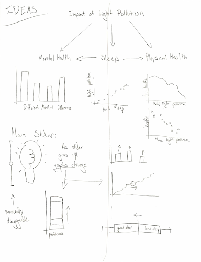
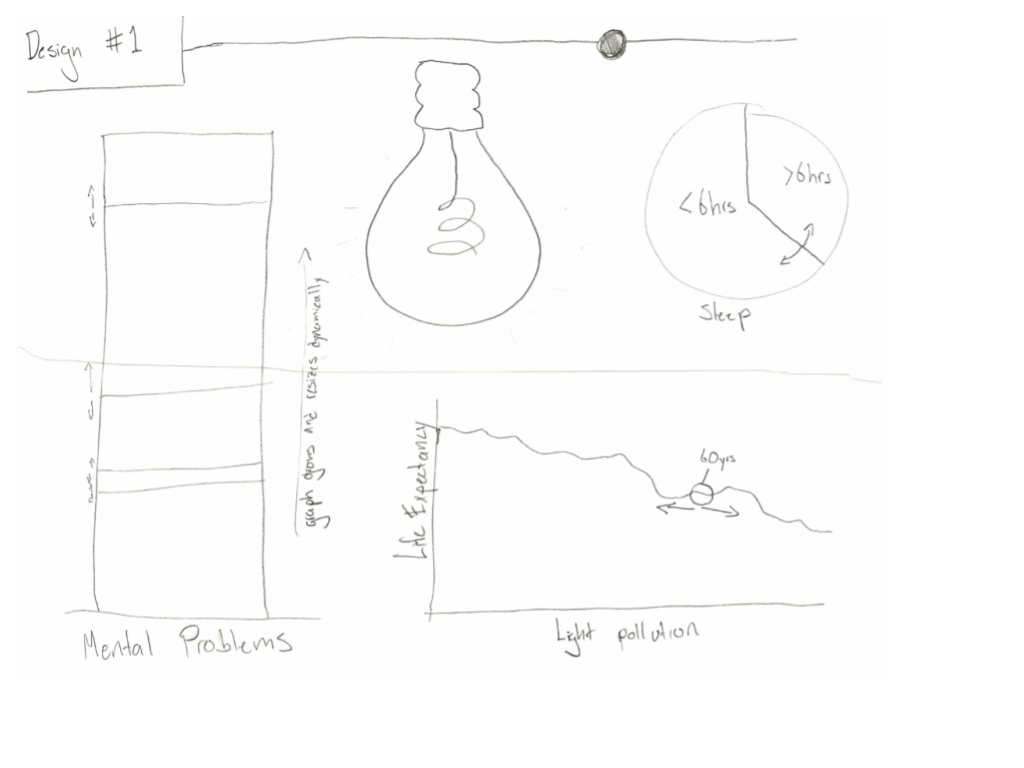
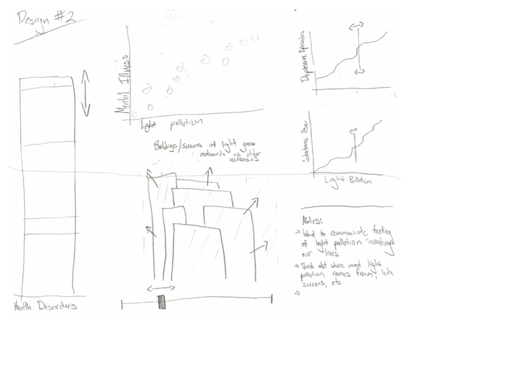
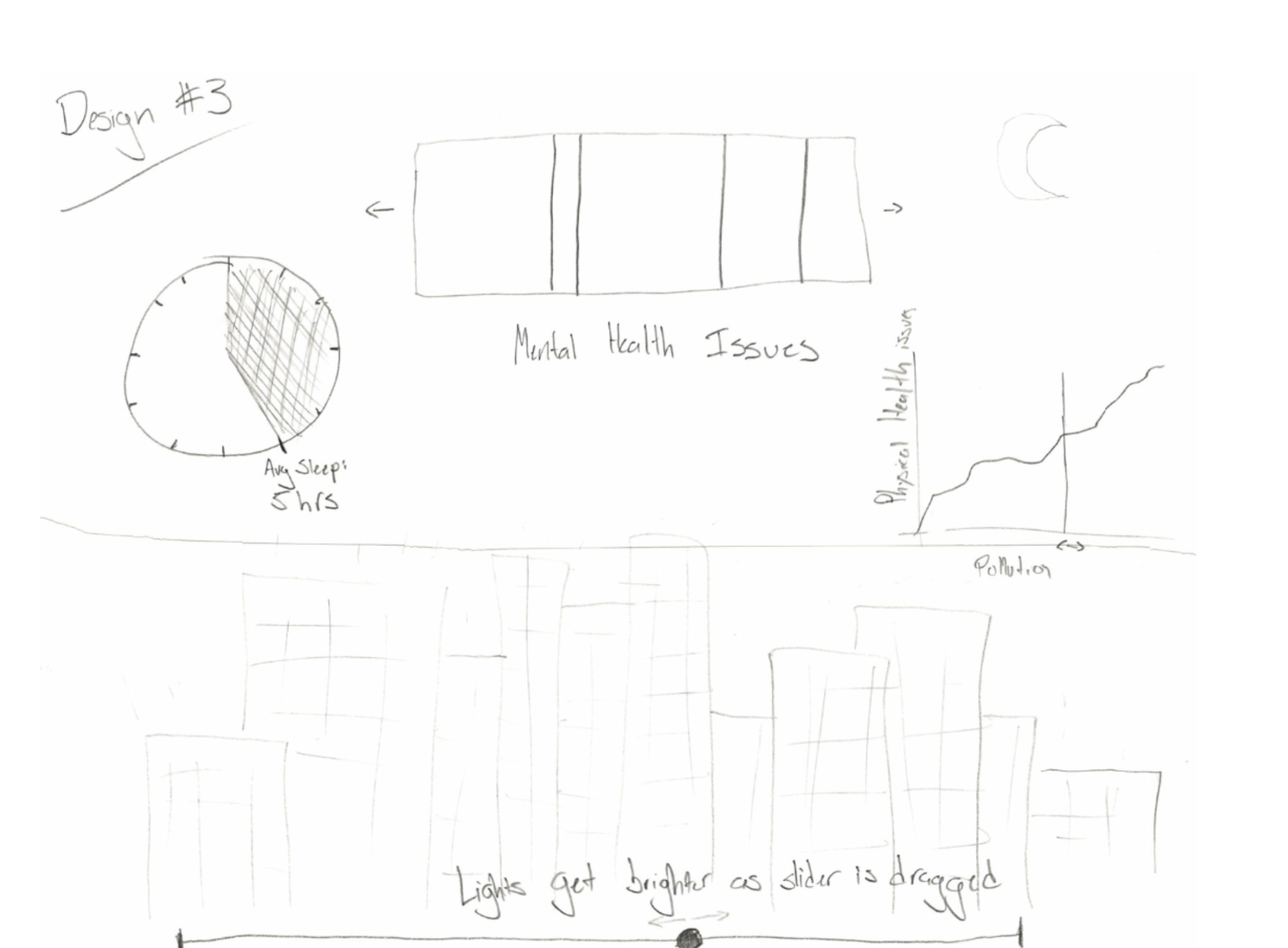
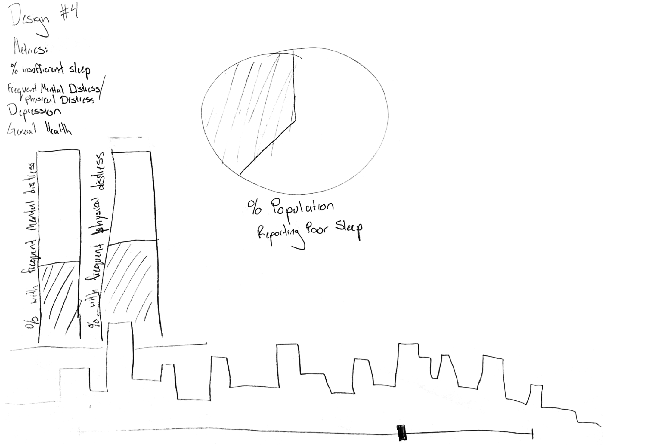
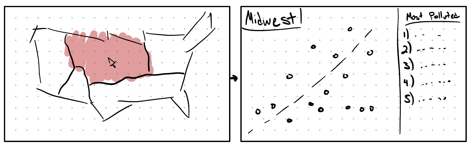
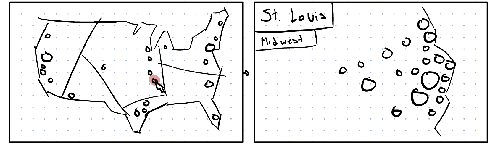
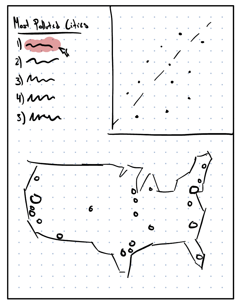
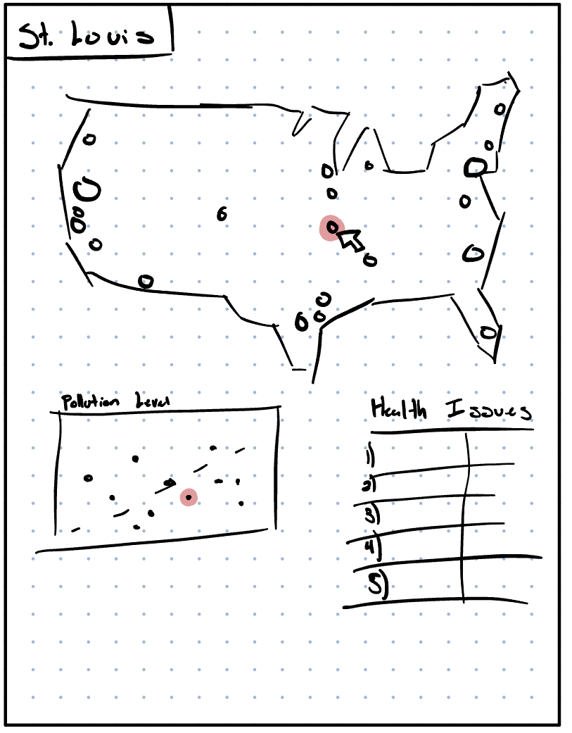
Below are the original designs from our brainstorm:
Originally we planned to have a vertical slider that will change the level of light pollution examined. With our multiple charts, the slider was supposed to populate the data to showcase the counties that exhibit the associated level of light pollution. Additionally, the slider was supposed to the background color (clear sky to cloudy sky) and other purely visual elements.
We also planned on bar charts, pie charts, and scatterplots to visualize the data. These charts change with the dropdown menu that isolates a specific health variable.
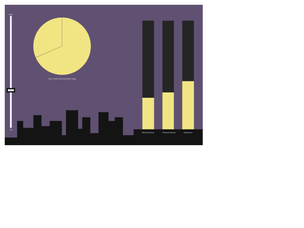
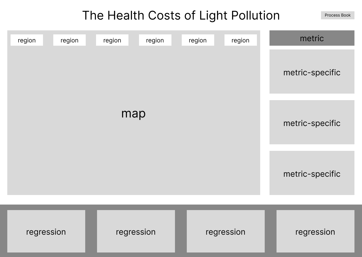
Milestone 1:
Milestone 2:
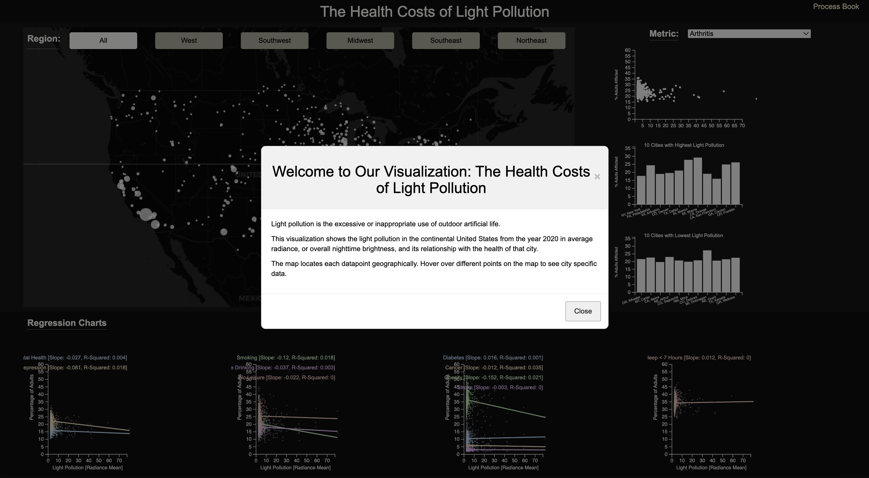
We then wanted to demonstrate an association between light pollution and health, so we added regression plots. We also replaced the slider with a selection tool that groups the data by regions of the United States. Finally, we added a welcome box, hints for the user on the website, and a short sentence involving our own conclusion.
We decided a dasboard layout was best in order for all the graphs to be visible at once. And we decided to keep the night-theme.
Sketches
As our design evolved, we prioritized the user's understanding and how the visualization answers the questions. The regression plots were added to better answer the questions of association between light pollution and health. The helpful hints and dashboard structure were added to make the visualization easier to interact with.
Implementation.
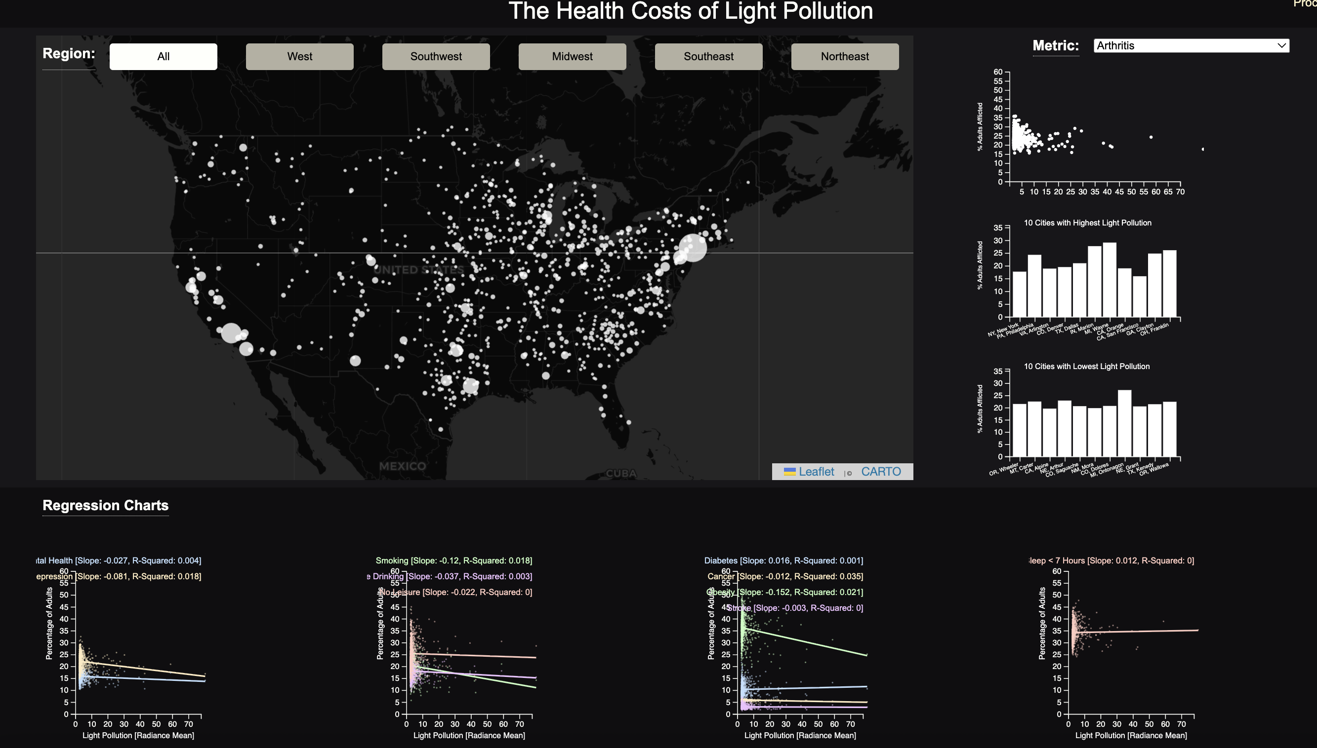
Our implementation has the following characteristics. You can select a particular region (West, Midwest, Northeast, Southwest, Southeast, or keep it set to Everything), and it will update the data displayed in all charts on the webpage to reflect the selected region.
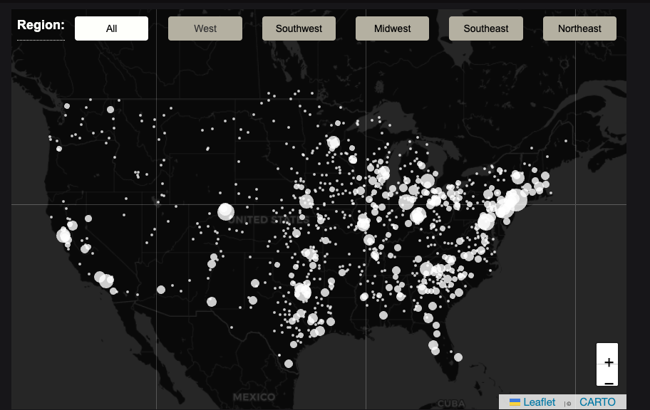
On our webpage, we have three major sections: map, regression charts, and metric specific charts. Map) Our map displays the cities from the chosen region by the user.
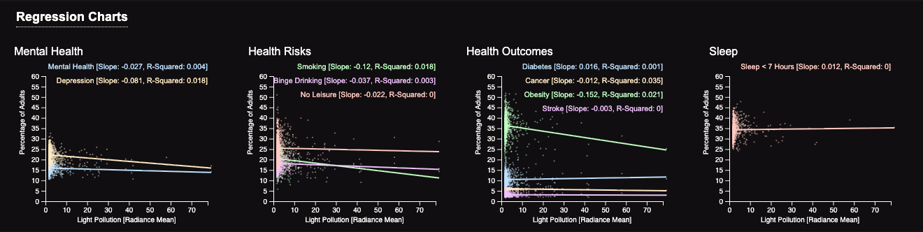
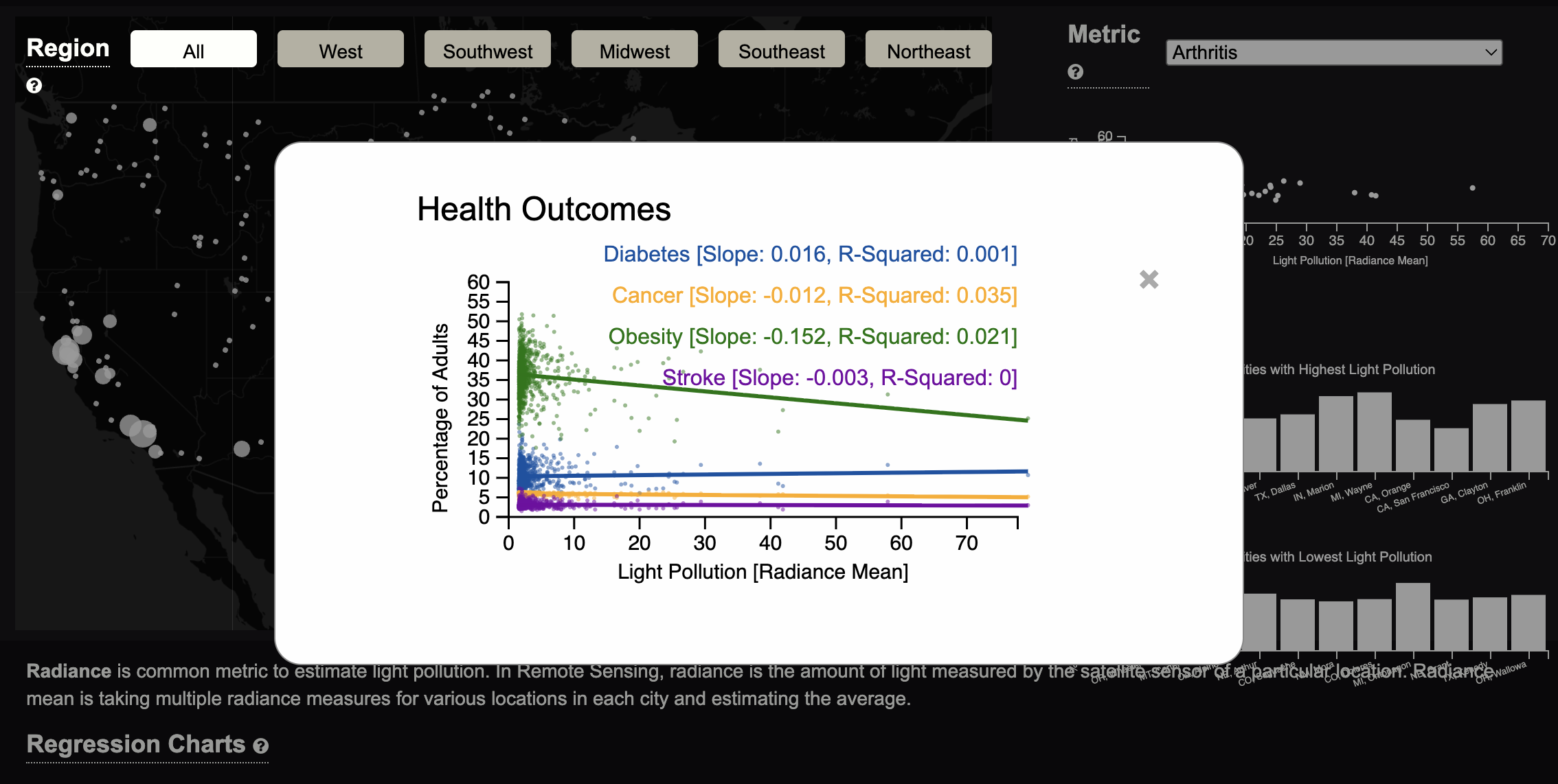
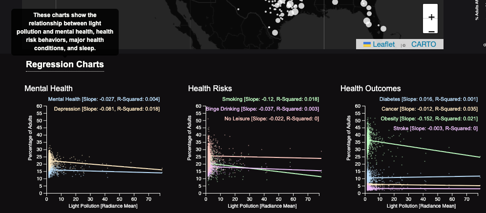
Regression Charts: This section features regression plots from left to right: mental health-related variables, health risk variables, key health outcomes variables, and lack of sleep.
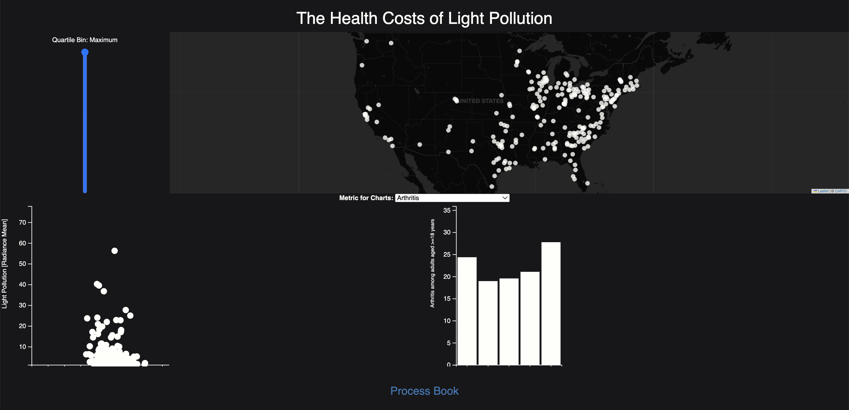
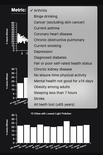
Metric Specific Charts: This section includes a scatterplot, a bar chart of the 10 cities with the highest light pollution, and another bar chart of 10 cities with the lowest light pollution. In addition, further interaction can be performed by selecting a particular variable from the dropdown in the section.
You can also expand a specific chart, the data, axis labels, and title will appear larger, and the plot is easier to see because there is not as much of a color contrast.
In many sections, helpful hints and insights can be found either through hovering over an icon, an overarching pop-up, and sentences within a section. Hovering your mouse over a heading with a dotted line will provide extra hints and insight.
Evaluation.
Through our visualization, we learned that there is not a strong association between health and light pollution. We answered the questions by making regression plots of different health conditions and light pollution. The first plot shows the association between health pollution and mental health, the second is physical health conditions, and the last is sleep. Through the directions of the lines, slope, and r-squared values, it can be seen that there is not an association between these health conditions and light pollution.
Our visualization works very well, particularly in how the different charts interact with each other. One thing we heard from users during the user study was that certain text and charts are too small and difficult to see. We improved this by implementing a maximizing feature where when you click a chart, it takes up more of the screen (is maximized on top of the other charts) and the color scheme changes. Another piece of feedback we got from our user studies was that it is difficult to find specific cities. A way the visualization could be improved is to have a search feature on the map that directs you to a specific city.